Quench Spectroscopy: A Step-By-Step Guide
A complete worked example of local quench spectroscopy
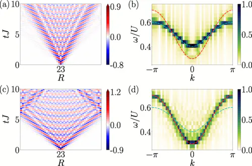 One of the colourful results from our paper!
Last week, I had a very nice exchange of e-mails with a PhD student interested in reproducing some results from a paper that I worked on, together with Louis Villa, Julien Despres and Laurent Sanchez-Palencia. The topic of the paper was local quench spectroscopy, a new technique that we proposed in 2020 for experimentally measuring the excitation spectrum of a quantum system by performing a quantum quench and observing the resulting dynamics. (There was also an earlier paper from the group using global quenches which I wasn’t involved with, and two later papers focused on disordered systems that I was involved with - for a full list of papers on the topic, see the end of this post!)
As part of this discussion, I put together a short exact diagonalisation code that outlined the main steps of a numerical simulation performing local quench spectroscopy, making use of the excellent QuSpin package, and I thought I’d take this opportunity to turn it into a brief blog post going through the anatomy of a quench spectroscopy calculation.
Background
Classical waves moving in a medium exhibit a property called dispersion, where waves of different wavelengths propagate with slightly different velocities, which gives rise to a mathematical quantity called the dispersion relation that links the wavenumber (momentum) of a wave with its frequency, which enables calculation of the group and phase velocities of a wavepacket. That might sound a bit dry, but think of light passing through a prism, or the famous Pink Floyd album cover - white light goes in, but because each of the different frequencies of light travel at different velocities, they all pass through the prism a little differently and exit at different points, resulting in a rainbow of different colours.
Quantum particles exhibit wave-like behaviour, and indeed excitations in quantum systems can also be described by a dispersion relation. As described by the Wikipedia page:
In the study of solids, the study of the dispersion relation of electrons is of paramount importance. The periodicity of crystals means that many levels of energy are possible for a given momentum and that some energies might not be available at any momentum. The collection of all possible energies and momenta is known as the band structure of a material. Properties of the band structure define whether the material is an insulator, semiconductor or conductor.
There are many ways to theoretically calculate dispersion relations, but experimentally it’s extremely challenging. One of the most well-established ways to do it involves measuring a quantity called the dynamical structure factor, which in practice involves measuring two-time correlation functions (i.e. given the state of a quantum system at a time t1, how similar is the state at a later time t2?), but this can be difficult, particularly in ultracold atomic gases where the measurements are typically destructive, i.e. once you measure the system once, you destroy the state that’s being measured, so it’s impossible to measure it again at a later time. So, can we come up with an alternative way of measuring dispersion relations of excitations in ultracold atomic gases?
The answer, of course, is ‘yes’! I’ll leave a list of papers at the bottom of this post to check out if you want the full details as to how it works, but here I’ll try to give you an intuitive explanation, followed by the code so you can see it in action for yourself.
The basic idea is the following: if we prepare the system in its ground state and then perform a quench to create a non-zero number of the excitations whose properties we want to measure, then by observing the resulting non-equilibrium dynamics, we can watch how the excitations move throughout the system. This gives us a picture of how the excitations move in space and time. The dispersion relation, however, relates the momentum of an excitation to its frequency. But we know that real-space and momentum are related to each other by Fourier transforms, and we know that frequency and time are related to each other by Fourier transforms. So in other words, if we observe the non-equilibrium dynamics in space and time, we can obtain the dispersion relation by making a 2D Fourier transform of the data!
There are of course some caveats here - we need to first create a state which contains the excitations we want to measure, then we need to pick an observable capable of measuring their dynamics. I’ll leave these subtleties out of the following, and suggest that if you’re interested, you check out some of the papers listed at the end of this post. Here, I’m going to instead walk you through an example of a numerical simulation of a transverse field Ising model, where the excitations are spin flips, and show you how to compute the non-equilibrium dynamics following a local quench (a single spin flip) and extract the excitation spectrum, then compare it to the exact known solution and see how well it agrees. This model can be solved exactly, so it’s a good test system to use to illustrate the method. (In the paper, we also looked at the more complex Heisenberg and Bose-Hubbard models.)
Code
The following code is written in Python, tested using Python 3.9.7 on a Macbook Pro (2021). The numerics for our paper were performed using the TenPy library, which allowed us to use matrix product state methods to reach large system sizes, but here I’ll demonstrate the method on smaller systems using exact diagonalisation, which can be run in a few seconds on a modern laptop. (Consequently, none of the below code was used for our paper, and all was custom written for this blog post and the discussion I had last week with a PhD student. I stress this because I’m not allowed to share the original code used in the paper.)
We start by importing the relevant packages:
#==============================================================================
# Initialisation
#==============================================================================

from scipy import fftpack
import numpy as np
import matplotlib.pyplot as plt
from quspin.operators import hamiltonian
from quspin.basis import spin_basis_1d
from quspin.tools.block_tools import block_ops
These packages are all standard (SciPy, NumPy, matplotlib), except possibly QuSpin which is a little more specialised but very useful, and it’s easy to download and install. If you use Anaconda, you can just type conda install -c weinbe58 quspin.
Next up, we initialise the parameters that we’re going to use. We’ll set up a transverse field Ising model of size L=11, with a spin-spin coupling J0=1 and an on-site field h=3, such that the ground state of the system is in the fully polarised state.
#==============================================================================
# Define variables
#==============================================================================
L = 11                          # System size
                                # Use odd numbers so the flip is on the central spin
J0 = 1.                         # Kinetic term (\sigma^x_i * \sigma^x_{i+1})
h = 3.                          # On-site term (\sigma_z)
Now we’ll use QuSpin to build the Hamiltonian, which can be done like so:
# Create site-coupling lists for periodic boundary conditions
J = [[-J0,i%L,(i+1)%L] for i in range(L)]
hlist = [[-h,i] for i in range(L)]

# Create static and dynamic lists for constructing Hamiltonian
# (The dynamic list is zero because the Hamiltonian is time-independent)
static = [["xx",J],["z",hlist]]
dynamic = []

# Create Hamiltonian as block_ops object
# This splits the Hamiltonian into different momentum subspaces which can be diagonalised independently
blocks=[dict(kblock=kblock) for kblock in range(L)]     # Define the momentum blocks
basis_args = (L,)                                       # Mandatory basis arguments
basis_kwargs = dict(S='1/2',pauli='1')
H_block = block_ops(blocks,static,dynamic,spin_basis_1d,basis_args,basis_kwargs=basis_kwargs,dtype=np.complex128,check_symm=False)
This initialises the Hamiltonian in terms of Pauli matrices, but spin operators can be used instead by changing the pauli='1' line to pauli='0'. The block_ops construction is used to split the Hamiltonian into different momentum-space blocks, which avoids having to build the entire Hamiltonian as a large matrix and lets use access slightly larger system sizes than we’d be able to reach otherwise. (To get to even larger system sizes, you can also restrict the basis to a particular magnetisation sector - in fact, for this model, we can restrict to the sector containing a single spin flip and simulate very large system sizes indeed, as it basically reduces to a single particle problem, but I’ll keep the following a little more general.)
Following our paper, I want to make a measurement of the Pauli y operator on every lattice site, so now I set up the operator using the hamiltonian class.
# Create the 1D spin basis
basis = spin_basis_1d(L,S='1/2',pauli='1')
# Set up list of observables to calculate
no_checks = dict(check_herm=False,check_symm=False,check_pcon=False)
n_list = [hamiltonian([["y",[[1.0,i]]]],[],basis=basis,dtype=np.complex128,**no_checks) for i in range(L)]
According to the scheme set out in our paper, I should at this point initialise the system in its (fully polarised) ground state and apply a local operator to rotate the central spin into the x-y plane. Here I’m going to do something a bit different and bit easier. As we’re quite far into the polarised phase, I can approximate the ground state as a product state with all spins pointing up, i.e. the |1111….> state in the notation of QuSpin. Rather than applying a local operator, I can initialise the system in an equal superposition of the states |1111…> (approximately the ground state) and |11…101…11> (the ground state with a spin flip on the central site). This means that the central spin is pointed somewhere in the x-y plane. (Note that this will work only sufficiently far into the polarised phase!)
We can do this using the following code snippet:
# Define initial state as superposition of two product states in the Hilbert space
# (This is equivalent to the spin rotation, but it's easier to do it like this in the ED code.)
st = "".join("1" for i in range(L//2)) + "0" + "".join("1" for i in range(L//2))
iDH = basis.index(st)
st_0 = "".join("1" for i in range(L))
i0 = basis.index(st_0)
psi1 = np.zeros(basis.Ns)
psi1[i0] = np.sqrt(0.5)
psi1[iDH] = np.sqrt(0.5)
Now that we’ve set up the initial state with a rotated central spin, next we have to time-evolve our state and compute the desired observable (as a reminder, the Pauli y operator on every lattice site). We can do that in the following way, here using a maximum time of t0=20 (implicitly in units of the spin-spin coupling J0) and 150 timesteps.
# Time evolution of state
times = np.linspace(0.0,20,150,endpoint=True)
psi1_t = H_block.expm(psi1,a=-1j,start=times[0],stop=times[-1],num=len(times),block_diag=True)

# Time evolution of observables
n_t = np.vstack([n.expt_value(psi1_t).real for n in n_list]).T
We can plot the density dynamics in the space-time basis using the following code:
# Plot density dynamics
fig=plt.imshow(n_t[::-1],aspect = 'auto',interpolation=None)
plt.colorbar(fig, orientation = 'vertical',extend='max')
plt.show()
plt.close()
The n_t[::-1] is used to rotate the figure so that time flows from bottom to top. (This could alternatively be achieved by changing the origin of imshow.) This results in the following figure:
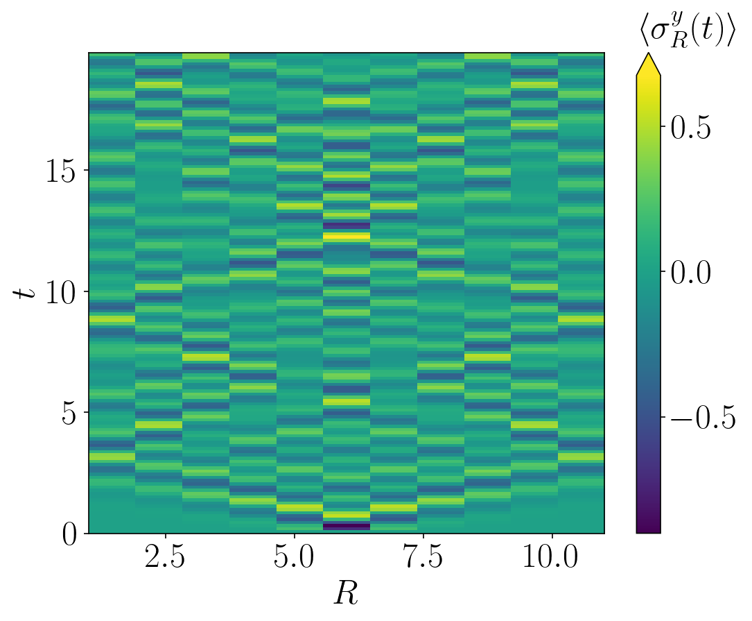
(Strictly speaking I should have modified the axis ticks as they’re a little off by default, but nevermind…)
For a small system like this, the ’light cone’ spreading of the initial excitation quickly hits the boundaries and reflects back from them, but it turns out that these reflections don’t cause significant problems in this system, so we don’t need to worry about them here. (Beware though, they can cause problems in others!)
Now we need to perform the 2D Fourier transform, which we can do using the built-in NumPy fft2 function. Notice here that there are a few tricky points to keep in mind. The first is that quench spectroscopy returns a signal at both positive and negative energies, so we use the fftpack library to compute the range of frequencies probed by this method so that we can label the final plot correctly. The second point is that the built in Fourier transform routines return the result in a way that isn’t very useful to us, so we use the fftshift function to rearrange the result in order from negative to positive frequencies.
The Fourier transform code is the following:
steps = len(times)
dt = times[1] - times[0]
# Compute Fourier transform of observables, and lists of momenta/energies
ft = np.abs(np.fft.fft2(n_t, norm=None))
ft = np.fft.fftshift(ft)
energies = fftpack.fftshift(fftpack.fftfreq(steps) * (2.*np.pi/dt))
# Normalise FT
data = np.abs(ft)/np.max(np.abs(ft))
At this point, we’re almost there - all we need to do now is calculate the exact result for the spectrum to compare our results to, and plot the data with the exact result overlaid on top of it. This can be done using the following code:
# Compute the exact result for the spectrum for plotting purposes
spectrum = np.zeros(L)
krange = np.linspace(-np.pi,np.pi,L)
for i in range(L):
    spectrum[i] = 2*np.sqrt(h**2+J0**2-2*h*J0*np.cos(krange[i]))

# Plot 2D Fourier transform
plt.imshow(data[::-1], aspect = 'auto', interpolation = 'none' , extent = (-np.pi, np.pi, max(energies)/J0, min(energies)/J0))
plt.plot(krange,spectrum,'r-')
plt.plot(krange,-1*spectrum,'r-')
plt.show()
plt.close()
This results in the following plot, where the density plot shows an object called the quench spectral function (QSF), and on top we plot the exact dispersion relation in red dashed lines. As you can see, they match perfectly! (Sidenote: we actually developed some techniques to get even cleaner data, but they’re too complex to go into here. They’re detailed in some of our later works, if you want more information.)
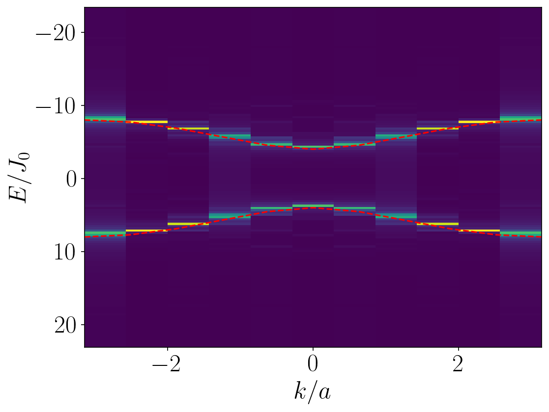
And there you have it - that’s how to do a quench spectroscopy calculation, where we have made use of local quench spectroscopy to extract the dispersion relation of the transverse field Ising model in the ferromagnetic phase, simply by rotating the central spin, observing the resulting dynamics and Fourier-transforming the final data. This code is available as a single Python script from my repository on GitHub.
For more information on quench spectroscopy using either local or global quenches, you can check out the following papers:
- Spectroscopy of Collective Excitations in Interacting Low-Dimensional Many-Body Systems Using Quench Dynamics, by Vladimir Gritsev, Eugene Demler, Mikhail Lukin, and Anatoli Polkovnikov, Phys. Rev. Lett. 99, 200404 (2007)
- Spectroscopy of Interacting Quasiparticles in Trapped Ions, by P. Jurcevic, P. Hauke, C. Maier, C. Hempel, B. P. Lanyon, R. Blatt, and C. F. Roos, Phys. Rev. Lett. 115, 100501 (2015)
- Quench dynamics of quantum spin models with flat bands of excitations, by Raphaël Menu and Tommaso Roscilde, Phys. Rev. B 98, 205145 (2018)
- Unraveling the excitation spectrum of many-body systems from quantum quenches, by Louis Villa, Julien Despres, and Laurent Sanchez-Palencia, Phys. Rev. A 100, 063632 (2019)
- Local quench spectroscopy of many-body quantum systems, by L. Villa, J. Despres, S. J. Thomson, and L. Sanchez-Palencia, Phys. Rev. A 102, 033337 (2020)
- Quench spectroscopy of a disordered quantum system, by L. Villa, S. J. Thomson, and L. Sanchez-Palencia, Phys. Rev. A 104, L021301 (2021)
- Finding the phase diagram of strongly correlated disordered bosons using quantum quenches, by L. Villa, S. J. Thomson, and L. Sanchez-Palencia, Phys. Rev. A 104, 023323 – Published 27 August 2021
- Louis Villa’s PhD thesis (2021)
Dr Steven J. Thomson
EPSRC Open Fellow, University of Edinburgh
Theoretical quantum condensed matter physicist, currently an EPSRC Open Fellow at the University of Edinburgh.